Exploring Galactic Cosmic Rays in the Heliosphere

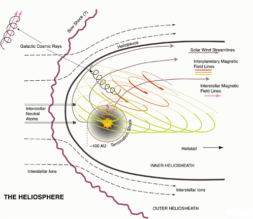
Heliosphere and Heliosheath

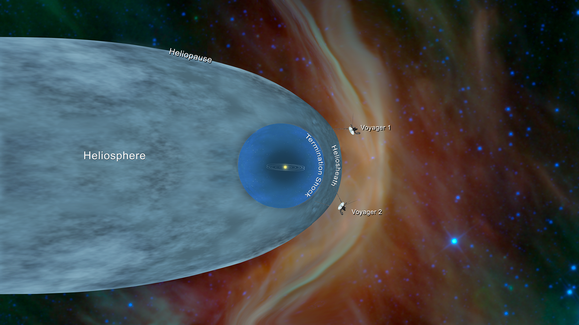
The heliosphere acts like a protective shield for our solar system, shielding us from high-speed charged particles in outer space that affect our life on Earth and space exploration. The Sun’s atmosphere is continuously expanding into space, forming a wind, known as the solar wind. Far from the Sun, at about 85-100 Astronomical Units (AU), far beyond the orbit of Pluto, the solar wind is slowed and heated by a large spherical-like structure known as the termination shock. Even farther away from the Sun, at the edge of the heliosphere, there is another large structure known as the heliopause, where the, now very weak solar wind meets the incoming interstellar material. Between these two structures, or boundaries, is a region of space known as the heliosheath, which contains slowed and heated solar wind. Beyond the heliopause is the local interstellar medium. The heliosphere may also have a massive bow wave where the interstellar material first interacts with the effects of our heliosphere. These are all transition regions, structures, and boundaries caused by the Sun’s interaction with the surrounding interstellar material. These regions and boundaries are important for understanding how our Sun interacts with the wider space around it. Spacecraft like Voyager 1 and Voyager 2 have given us valuable information about the heliosphere, helping scientists learn more about its boundaries. Check out the particle fluxes including galactic cosmic rays (GCRs) on the Voyager CRS Flux Time History page!

Energetic particles play a crucial role in shaping the dynamics of the plasma universe. Within the heliosphere, which acts like a smaller version of the larger plasma universe, lots of high-energy activities happen, even if they are not as intense as elsewhere in the Universe. Because of their high speeds, approaching the speed of light, they are very mobile and are useful probes for exploring what is happening in different parts of the heliosphere, including near the Sun itself which accelerates particles to high energies in large solar explosions such as flares and coronal mass ejections. The contributions of Ulysses, Advanced Composition Explorer (ACE), Solar and Terrestrial Relations Observatory (STEREO), and Parker Solar Probe (PSP) have been instrumental in advancing our comprehension of the heliosphere’s dynamics and the behavior of energetic particles as well. By studying the heliosphere, scientists learn about other parts of the plasma universe too since the basic science of particle acceleration and transport can be studied up close.

Solar wind and magnetic field

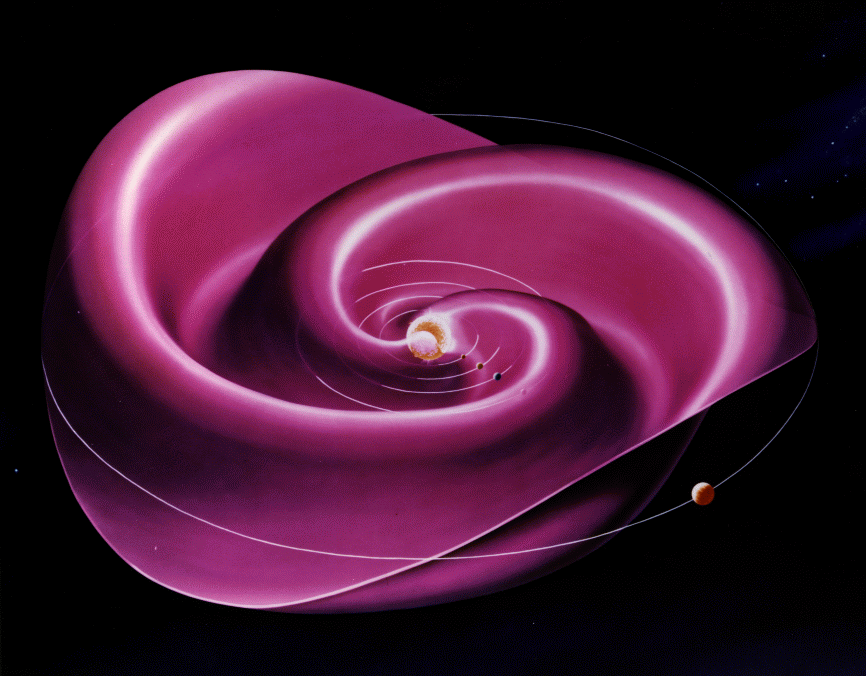
Back in 1958, a scientist named Eugene Parker came up with the term “solar wind”. It’s a fascinating phenomenon that happens because of charged particles like electrons, protons, and alpha particles moving outward from the Sun’s outer atmosphere, called the corona. Now, the corona has open and some closed magnetic field lines. The open ones, mainly in the polar regions, sometimes stretch towards the equator, linking the Sun’s surface with the interplanetary space. These open lines are like the starting point for what we call the “fast solar wind”.

Picture this: the solar wind carries the magnetic field from the corona into the heliosphere, forming something called a heliospheric current sheet that fills the heliosphere. The Sun’s magnetic field and its rotation play a role in shaping this sheet and influencing where the solar wind is stronger or weaker. The current sheet, by definition, separates the heliosphere into regions with different magnetic field polarities. Because of the Sun’s rotations, this sheet moves up and down from the perspective of a fixed observer, giving it a kind of “ballerina skirt” effect.

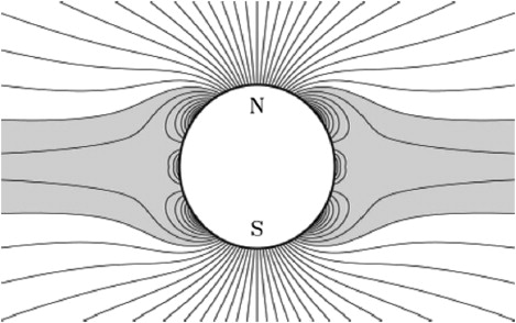
Potential-Field Source-Surface (PFSS) model

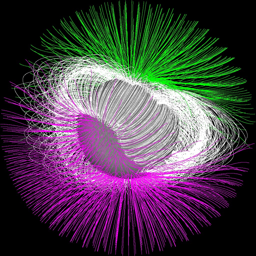
Every 11 years, the Sun’s magnetic field goes through a fascinating reversal. Understanding this process is crucial for anticipating potential severe space weather conditions. A handy tool for grasping this phenomenon is the Potential- Field Source-Surface (PFSS) model, known for its simplicity and effectiveness in depicting the large-scale coronal magnetic field.

This model, initially developed in 1696 by Kenneth H. Schatten, John M. Wilcox, and Norman F. Ness, has been refined over the years by various scientists. Here’s how it works: solar magnetograms, like those captured by instruments such as SOHO/MDI and SDO/HMI, provide the magnetic field at the inner boundary, while the “source surface” provides the outer boundary. The source surface is a sphere around the Sun where the magnetic field is prespecified, and is usually taken to point either away from or towards the Sun (i.e. a “radial field”). Generally, the radius of the source surface is assumed to be about twice that of the Sun, but this is an adjustable parameter.

This model is based on a current-free approximation of the solar corona. This simplification enables us to describe the magnetic field as a gradient of a scalar potential. By applying Gauss’s law, we arrive at the Laplace equation. The 3 solutions of the Laplace equation can be expressed in the form of spherical harmonics. Another key aspect of this model is the assumption that the magnetic field is purely radial at the source surface. In simpler terms, the model simplifies things to make it easier to understand and still captures the essential aspects of the Sun’s magnetic behavior.

Adapted from “Potential-Field Source-Surface Models” from NSO, and from “On Solutions of the PFSS Model With GONG Synoptic Maps for 2006–2018” from Ljubomir Nikolic on “Space Weather”, Volume 17 (2019).

Galactic Cosmic Rays

Among the many types of energetic particles swirling around in the heliosphere, like the Solar Energetic Particles (SEPs), Galactic Cosmic Rays (GCRs) stand out. GCRs have been a big deal in space science since they were first spotted by V. F. Hess in 1912 during balloon flights.

GCRs are characterized by their high energies reaching up to 10¹⁷ eV.They do not come from our Sun though. Instead, most of them likely originate from the shock waves around exploded massive stars, called supernovae, outside our solar system. The ones at the highest energies are not well understood and may even come from outside our galaxy. Traveling through the galaxy, they are guided by its magnetic field and get jostled around by turbulence. It takes about 10 million years for them to make their way into our solar neighborhood. But once they are here, they are not just free to roam. The solar wind and heliosphere act as a barrier to them, and their intensity is reduced. The Sun’s magnetic activity and “sunspot cycle” can affect their intensity. When the Sun is at its most active, GCRs are at their minimum.

Although it is plausible that GCRs can originate from supernova remnants, they cannot reach the highest energy we observe above 10¹⁶ - 10¹⁷ eV. This energy limit shows up as a "knee" in their energy spectrum around 10¹⁵ eV. The most energetic GCRs either get a boost in energy from within our Galaxy, come from outside it altogether, or even shoot out from objects like young pulsars.

Studying these energetic particles is not just about understanding high-energy astrophysics. It led to the discovery of new subatomic particles, drawing the attention of big names in physics like John Simpson, Frank McDonald, and James Van Allen.

Adapted from "Acceleration of Energetic Particles on the Sun, in the Heliosphere, and in the Galaxy" from Martin A. Lee on "Acceleration and transport of energetic particles observed in the heliosphere" (ACE-2000 Symposium).

Force-field approximation (FFA)

When cosmic rays from space approach the Sun, they undergo changes because of their interaction with the solar wind and the Sun’s magnetic field. These changes are linked to the solar activity variation, and we call this process “solar modulation” for GCRs.

In 1965, Eugene Parker described these changes using the Parker transport equation. This equation helps us understand how cosmic rays move in space around the Sun. However, the Parker transport equation is quite complex, making it challenging to solve directly. To make things simpler, scientists often use the force-field approximation (FFA), first proposed by Gleeson and Axford in 1968. This simplified model assumes that the space around the Sun is spherically symmetric, and everything stays relatively constant over time (steady-state heliosphere). In this imaginary bubble, there are no specific places where cosmic rays are either created or disappear. The focus is only on how cosmic rays move toward or away from the center (the radial direction). Additionally, adiabatic energy losses that might happen when cosmic rays interact with the changing environment around the Sun are not considered. Instead, things are further simplified by considering a diffusion coefficient that depends only on the distance from the Sun and the momentum of the GCRs.

The force-field approximation provides a simpler way to study the large-scale features of GCRs’ movement around the Sun. However, it’s important to note that this simplified model ignores some of the intricate details present in the full Parker transport equation. This simplification is acceptable when researchers are mainly interested in understanding broader trends and characteristics of GCRs near the Sun, rather than getting into specific local effects like GCR drifts.

Adapted from “Comprehensive modulation potential for the solar modulation of Galactic cosmic rays” from Xiaojian Song, Xi Luo, Marius S. Potgieter, Ming Zhang on “Physical Review D.” (2022), and from “Uncertainties implicit to the use of the force-field solutions to the Parker transport equation in analyses of observed cosmic ray antiproton intensities” from N. Eugene Engelbrecht and Valeria Di Felice on “Physical Review D.” (2020).

Diffusion coefficients

GCRs move around in space in two main ways: they drift along the average magnetic field and also move randomly, a process called diffusion. This diffusion is an essential part of the equation describing how GCRs move (the Parker transport equation). Diffusion can be broken down into two types: parallel diffusion, which happens along the direction of the magnetic field, and perpendicular diffusion, which occurs across the field. Usually, parallel diffusion is stronger than perpendicular diffusion.

When there’s no turbulence, GCRs just follow the magnetic field lines. But in turbulent conditions, they start to move more chaotically, crossing magnetic field lines and changing direction. The turbulence in the solar wind and heliosheath is closely linked to diffusion. The strength of the magnetic field (and the turbulence) directly (inversely) affects the parallel diffusion and inversely (directly) affects the perpendicular diffusion.

To create an accurate model, we need to understand diffusion throughout the entire heliosphere. Arguably, the most important factor is the perpendicular diffusion coefficient, since field lines are tightly wound, and both radial and latitudinal diffusion are controlled by this coefficient beyond a few tens of AU. The perpendicular coefficient is also the most challenging aspect for scientists to study and predict.

Understanding how GCRs move is a complex task, and it depends on the patterns and strength of magnetic fields and turbulence in space. Exploring the diffusion of these cosmic rays is vital for understanding how they travel through the heliosphere.

Adapted from “Cosmic Rays in the Heliosphere” from Bernd Heber, Jozsef Kota, Rudolf von Steiger on “Space Sciences Series of ISSI”, Springer (2013).

The History at LPL

The Solar and Heliospheric group of this department has been delving into the mysteries of cosmic ray transport for quite some time. One of the leading figures in this journey was Professor Randy Jokipii, a true trailblazer in the field. Not only has he laid the groundwork but also set up essential frameworks for understanding how cosmic rays get influenced as they journey through the heliosphere.

One of his groundbreaking contributions was linking the power spectrum of magnetic fluctuations to the cosmic-ray diffusion coefficients. This is crucial for grasping a whole range of phenomena in space, like how cosmic rays get affected as they travel through our solar system. Later, together with Professor Joe Giacalone, they performed extensive numerical studies to simulate the transport of charged particles in stochastic magnetic fields with realistic spectra and derive the principal components of the diffusion tensor.

Professor Jokipii was also ahead of his time in interpreting the 22-year cosmic ray cycle. He explained how the flipping of the Sun’s magnetic state every 11 years results in different cosmic ray profiles in even and odd solar cycles, repeating every 22 years.

Working alongside him was his esteemed colleague, Dr. Jozsef Kota, who made significant strides in the field as well. Professor Jokipii, with Dr. Kota, was the first to point out the importance of transverse magnetic fluctuations that profoundly affect particle transport in the polar regions of the heliosphere. Dr. Kota developed various numerical codes to simulate how GCRs travel and change their energy within the interplanetary magnetic field. These simulations allowed them to explore even the most remote areas of the heliosphere. He also extended the models to capture more realistic scenarios and geometries, unlocking deeper insights into the cosmic ray transport happening all around us in space.

The SHIELD Program

The SHIELD DRIVE Science Center, an international collaboration led by Merav Opher from Boston University, is focused on understanding the protective bubble around our Solar System. Their ultimate goal is to create a detailed model of the heliosphere using a combination of observations, modeling, and theory. The center explores various aspects, including how cosmic rays travel through the heliosphere, the overall structure of the heliosphere, and how it interacts with the local interstellar medium. Additionally, the center investigates the impact of pickup ions on the processes occurring within the heliosphere.